Contents
See also external module loadModelData.m this file: demoDataGen.m data files: FakeData.mat, FakeData.csv.
Generate model data in 2D
Consider N + (alpha * N) objects of two classes. Let objects be random, distributed normally, the multivariate random variable of the 1st class could be described by the unit diagonal covariance matrix, and 2nd’s by the matrix diag(sig2).
The simplest way to get data
The simplest and dirty way to get model data is to type them by hands in the code.
X = [0,1; 1,0];
y = [  0;   1];
Load from a mat or csv file
% the data could be loaded from external mat-file
% load FakeData.mat % file must contain X and y (do not forget - convention)
% or from Comma-Separated-Values worksheet
% dummy = dlmread('FakeData.csv', ',');
% X = dummy(:, 1:end-1); % this indices are under convention
% y = dummy(:, end);
% clear dummy % no needs to keep a big storage
Generate data by a module
The data could be generated by external module of special purpose
N = 100; % 1st class contains N objects
alpha = 1.5; % 2st class contains alpha*N ones
sig2 = 1; % assume 2nd class has the same variance as the 1st
dist2 = 4;
%
% % later we move this piece of code in a separate file
% [X, y] = loadModelData(N, alpha, sig2, dist2);
N2 = floor(alpha * N); % calculate the size of the 2nd class
cls1X = randn(N, 2); % generate random objects of the 1st class
% generate a random distance from the center of the 1st class to the center
% of the 2nd
ShiftClass2 = repmat( ...
    dist2 * [sin(pi*rand)  cos(pi*rand)], ...
    [N2,1]); %
% generate random objects of the 2nd class
cls2X = sig2 * randn(N2, 2) + ShiftClass2;
% combine the objects
X = [cls1X; cls2X];
% assign class labels: 0s and 1s
y = [zeros(size(cls1X,1),1); ones(size(cls2X,1),1)];
%end % of module
The given data are X and y
X is a matrix of (N1+N2 by 2), and y is an (N1+N2)-column vector. Indices for objects are very useful to deal with during the plot.
X; y; % note that y contains only 1s and 0s
idx1 = find(y == 0); % object indices for the 1st class
idx2 = find(y == 1);
% no more variables are needed
Preliminary plot
Plot the given data to observe possible obstacles to classification.
h = figure; hold on
plot(X(idx1,1), X(idx1,2), 'r*');
plot(X(idx2,1), X(idx2,2), 'b*');
axis tight
xlabel('x_1');
ylabel('x_2');
% close(h);

Classification: fit the algorithm parameters
Use a logistic regression as a classification algorithm to classify objects
bHat = glmfit(X,y,'binomial');
Classification: use the model
We have the model y = 1/(1+exp(-Xb)) and its parameters bHat. Use the model to get the estimations of class labels.
yHat = glmval(bHat, X, 'logit'); % variant of classification
yHat = 1./(1+exp( -[ones( size(X,1),1 ), X] *bHat)); % variant of classification
% formed as an inline function
classify = inline( '1./(1+exp( -[ones( size(X,1),1 ), X] *b))', 'b', 'X');
% separation hyperplane, formed as a function (here it is a line)
separateXLim = inline( '(-b(1)- YLim*b(3))/b(2)', 'b','YLim');

% example of classification model usage
yHat = classify(bHat,X);
Plot the results in 2D
% the objects could be surrounded by circles
idx1 = find(yHat < 1/2); % object indices for the 1st class
idx2 = find(yHat >= 1/2);
plot(X(idx1,1), X(idx1,2), 'ro');
plot(X(idx2,1), X(idx2,2), 'bo');
% or separated by plane
plot(separateXLim(bHat,YLim), YLim, 'b-');

Plot in 3D and save
To plot 3D surface of probability we should compute the probability function in each point of the X1 by X2 – plane.
% to do that create a grid
GRIDSIZE = 10;
linX1 = linspace(min(X(:,1)), max(X(:,1)), GRIDSIZE); % grid of feature values
linX2 = linspace(min(X(:,2)), max(X(:,2)), GRIDSIZE);
[grdX1 grdX2] = meshgrid(linX1, linX2); % cartesian product of two grid sets

grdX1 = grdX1(:); % vectorize the obtained matrices
grdX2 = grdX2(:);

Tri = delaunay(grdX1,grdX2); % make Delauney triangulation
trisurf(Tri,grdX1,grdX2,classify(bHat,[grdX1 grdX2])-1/2,...
'FaceColor','red','EdgeColor','none');
camlight left; lighting phong; % alpha(0.8);
% the plane was shifted down to 1/2

% to save the picture use the figure handle h
% saveas(h, 'demoDataGen_saved.png', 'png');
% saveas(h, 'demoDataGen.eps', 'psc2');
close(h);