This demo shows how to deal with the different hypothesis on data generation. The data generation hypothesis here is an assumption about the link function. We have a synthetic model and three link functions. We generate a sinthetic noise, denerated according to the correspondent hypothesis and to the link function. The problem is to find the model parameters and recover the dependent variable of the regression.
Contents
Make a synthetic data set
N = 1000;
% independent variable
x = linspace(-1,1,N)';
% the model
f = inline('[x.^2, x.^3, exp(x)]','x');
%$X = [x.^2 x.^3 exp(x)];
% model coefficients
b0 = [-1.5, -2, +1.3]';% + 7 ;
% make the dependent variable
X = f(x);
y0 = X*b0;
The normal distribution and the identity link function
distr='normal';
link='identity';

% append noise to the dependent variable
y = X*b0 + normrnd(0,1,N,1);

% recover the dependent variable
b = glmfit(X,y,distr)
y1 = glmval(b, X, link);

% plot the results
h = figure; hold on
plot(x,y,'.');
plot(x,y1);
plot(x,y0,'r-');
legend('source data', 'recovered function', 'initial function');
xlabel('x'); ylabel('y'); title('distribution is normal, link is identitiy');
saveas(h,'demo_GLM_1.png','png');
close(h);
b =

    0.3082
   -1.4866
   -1.5041
    1.0358

The gamma distribution and the reciprocal link function
distr='gamma';
% link='log';
link='reciprocal';

% the link function is reciprocal, gInverse == g
g = inline('1./Xb', 'Xb');
mu = g(X*b0);

% assign the distribution parameters
shape = 10.0;
scale = mu/shape;

% generate gamma distributed values with the given mean values
y = gamrnd(shape,scale);

b = glmfit(X,y,distr, 'link', link)
y1 = glmval(b, X, link);

% plot the results
h = figure; hold on
plot(x,g(y),'.');
plot(x,g(y1));
plot(x,y0,'r-');
legend('source data', 'recovered function', 'initial function');
xlabel('x'); ylabel('y'); title('distribution is gamma, link is reciprocal');
saveas(h,'demo_GLM_2.png','png');
close(h);
b =

   -0.0894
   -1.4666
   -2.1322
    1.3678

The normal distribution and the custom link function
distr='normal';
FL = inline('x.^.5');
FD = inline('.5*x.^-0.5');
FI = inline('x.^2');
link = {FL FD FI};

% append noise to the dependent variable
Mu = 17; % see the link and inverse link functions
y = FI(X*b0 + normrnd(Mu,1,N,1)) ;

% recover the dependent variable
b = glmfit(X,y,distr, 'link', link)
y1 = glmval(b, X, link);

% plot the results
h = figure; hold on
plot(x,FL(y),'.');
plot(x,FL(y1));
plot(x,y0+Mu,'r-');
legend('source data', 'recovered function', 'initial function');
xlabel('x'); ylabel('y'); title('distribution is gamma, link is y^{1/2}');
saveas(h,'demo_GLM_3.png','png');
close(h);
b =

   17.2253
   -1.4887
   -1.7157
    1.1815