Though our online index calculator that performs automatic index construction is suspended now, we briefly describe the project and provide instructions on building indices using our technics.
Introduction to an index construction
This educational project is devoted to the problem of index construction. The index is the most informative description of an object. So, there is a set of objects. A rating is an ordering of the set according to the indices of the objects. There are lots of ways to construct indices. However, when algorithms are chosen, and some results are obtained, the following question arises: how to show adequacy of the calculated indices?
To answer the question, analysts invite experts. The experts express their opinion, and then the second question arises: how to show that expert estimations are valid? There is a technique that produces valid indices based on measurement data and expert estimates.
Contents
Note: this is the first version of the index construction service. We apologize for any mistakes and would be grateful if you send us.
How to fill the template?
Before starting an index construction, you have to prepare the following information.
- A list of objects. You can use any names, but they should be short. Don’t use too many characters.
- A list features.
- Each feature must have a factor. The factor is either +1 or -1. It shows whether the bigger feature values correspond to the bigger values of indices (Factor = 1) or the smaller feature values correspond to the bigger values of indices (Factor = -1).
- A data table with no empty items.
Note the next simple facts:
- Are the objects comparable? If one object has much bigger or smaller values in one or several features than the others, the indices might be unstable. They could drastically change if you exclude this object from the list.
- Are the features completely describes the objects? You cannot make an index of a person’s intelligence quality using data on his vital statistics.
- The factor values are intended to adjust data to the principle: “the bigger the better”. If you make sport indices and use the features: Citius, Altius, Fortius (Faster, Higher, Stronger) then the Factor values are -1 (i.e. sprint, seconds), +1 (high jump, meters), +1, (weightlifting, kg), then the bigger values of the result indices will show the better sportsman.
- Data values should be linear (not ordinal) scaled. What does it mean? Assume one feature of the objects. If you feel free to make any arithmetic operation with object values, the values are in the linear scale.
Example one (feature has linear scale). The objects are cars, and the feature is weight. We can say that Car1 is twice lighter than Car2 if the first one has a value of 400 and the other has 800.
Example two (feature has ordinal scale). Objects are the same, and the feature is usability. We can say that Car1 is more convenient than Car2. However, we can not say it is twice more convenient.
If one uses features like those in the second example, he should be careful about the indices he obtains. For this type of scale, there are special algorithms like Pareto slicing.
The base algorithm for an index construction is Principal Components Analysis.
Using features weights
If one obtains an index of his data table and features weights, he can use the weights as a fixed model for indices computation. To make the next index based on the same set of objects and the same set of features, one has to do the following.
Denote the data table as m-by-n matrix A with items aij, where m is the overall objects number and n is the overall features number. Denote features weights as w1,…,wn and objects indices as q1,…,qm.
The index of i-th object is
qi = w1ai1+w2ai2+…+wnain.
This model can be used if the source data are lightly changed. The strong side is that if the changes were in a small number of objects, those objects whose data was not changed would keep their indices unchanged. The weak side is that the indices would be incorrect if there were drastic changes. Sometimes the, drastic changes can occur even if one object changes its feature. One must compute indices using changed data to decide whether one should use the weighting model. If one decides that new indices and weights vary too much, he must decline the old model’s weights.
SUMMARY
- Use this weighting model if there are little changes in your data and if you want to keep most objects’ indices unchanged.
- Do not use this model if there are drastic changes in your data./li>
File operations
For an index construction, you have to make the following steps:
- Download a template with object description data or create the template yourself.
- Fill the template with data. The data must be numbers.
- Upload the template back so the index are to be calculated.
- Check your table in View section and observe the Report section.
Get a template
There is only one template in the database for now. You can download it in the CSV text format. Also you can copy the data from the examples. Read further to learn how to fill the template.
Put your file to the index calculator
Now you should click the browse button to find the file on your computer and upload it. If the file is well-formatted, the system switches this tab to the View tab.
Template files example
You can upload either an XLS file or a CSV file. The first one has the following format. The special word “Factor” is reserved. It shows whether the bigger feature values correspond to the bigger values of indices (Factor=1) or the smaller feature values correspond to the bigger values of indices (Factor=-1). An XLS table example is below. You can select the whole table, copy it, open your MS Excel, click the mouse pointer to the worksheet cell A1 and paste it.
| Feature1 | Feature2 | Feature3 | |
| Factor | 1 | -1 | 1 |
| Object1 | 0,69 | 7,53 | 4,69 |
| Object2 | 0,69 | 7,53 | 7,38 |
| Object3 | 4,34 | 0,43 | 5,69 |
| Object4 | 8,48 | 8,37 | 5,29 |
| Object5 | 5,31 | 6,84 | 4,02 |
| Object6 | 7,08 | 0,96 | 4,02 |
| Object7 | 4,68 | 5,5 | 3,42 |
A CSV file (Comma Separated Values) is a text file. It contains the following lines.
, Feature1, Feature2, Feature3
Factor, 1, -1, 1
Object1, 0.69, 7.53, 4.69
Object2, 0.69, 7.53, 7.38
Object3, 4.34, 0.43, 5.69
Object4, 8.48, 8.37, 5.29
Object5, 5.31, 6.84, 4.02
Object6, 7.08, 0.96, 4.02
Object7, 4.68, 5.5, 3.42
The data is the same as in the table above. Note that the decimal points are dots, while the value separators are commas. You can select the whole table, copy it, open your Notepad or another text editor, and paste the table.
The index construction procedure
An index is the most informative description of data. We use Singular Value Decomposition and Principal Components Analysis to perform an index construction. It gives the indices that fit the source data the most precisely.
The first step is feature normalization. We need to de-scale data. The table below shows the measurement data for two scales: the scale of Feature1 and Feature2. We can not use the source scales since the values of Feature2 are two times bigger than the values of Feature1. In this case, our index will pay attention to the Feature2 data and ignore the Feature1 data. So we have to make both features to be on the same scale.
| Feature1 | Feature2 | Feature1 | Feature2 | ||
| Factor | 1 | 1 | |||
| Obj1 | 2.66 | 30.00 | 0.8300 | 0.0000 | |
| Obj2 | 1.00 | 44.63 | 0.0000 | 0.4877 | |
| Obj3 | 3.00 | 40.33 | 1.0000 | 0.3443 | |
| Obj4 | 1.98 | 50.50 | 0.4900 | 0.6833 | |
| Obj5 | 1.23 | 60.00 | 0.1150 | 1.0000 | |
| Obj6 | 2.49 | 34.55 | 0.7450 | 0.1517 | |
| Obj7 | 1.89 | 55.50 | 0.4450 | 0.8500 |
Let the scale be the segment [0,1]. The minimal value of a feature will be 0 while the maximal value will be 1 (so each feature has at least one 0-value and at least one 1-value). The formula of the normalization is the following. Denote aij a value of i-th object and j-th feature. Then the new value will be
The figure below shows the objects with normalized feature data. Objects are marked by asterisks. The main idea of the algorithm is the following. We find a vector called 1-st Principal Component (red segment in the figure). Projections of the objects given on the 1st PC show the maximal distribution. The Projections are denoted by dots. The object index is the distance from the point (0,0) to an object projection.

Index construction
The table below represents the object indices.
| Objects | Indices |
| Obj1 | 0.60 |
| Obj2 | 0.34 |
| Obj3 | 0.96 |
| Obj4 | 0.83 |
| Obj5 | 0.77 |
| Obj6 | 0.64 |
| Obj7 | 0.91 |
The feature weights are very informative data. The weight table shows that both features have approximately equal importance. However, there is data with different weight values. This information discovers what features have a great (or small) impact on indices.
| Features | Weights |
| Feature1 | 0.72 |
| Feature2 | 0.69 |
See also our article about expert-statistical techniques for index construction.
How our Ratings and Integral Indicators calculator works?
To run it please do the following.
1. Download Example.xls, use “Simple” sheet.
2. Put your Objects in the 1st column starting at A2.
3. Put your Features in the 1st row starting at B1.
4. If a bigger value of a Feature supposes a bigger value of the Rating (“the bigger the better principle”), put +1 right under the corresponding feature (the red row). Otherwise put -1.
5. Fulfill the data table.
6. Send your file back.
7. Within a minute you will have a Report on your Rating back.
If you would like to use more complex sheets, please write me. Find the introduction and the theory on the calculator.
Thanks for supporting our index construction project
The project devoted to index construction technics was supported by the Department of mathematical modeling in Ecology and Medicine of the Dorodnicyn computing center of the RAS.